行外人的一次 TCGA 数据库基因差异分析

请注意，本文编写于 1480 天前，最后修改于 1418 天前，其中某些信息可能已经过时。

自 2021 年 1 月开始，笔者跨学科参与医学院大创项目，在团队内负责生物信息学方向的工作。本篇博文主要记录寒假内的工作，即基于 TCGA 数据库的替莫唑胺 (Temozolomide, TMZ) 治疗脑胶质瘤 (Low Grade Glioma, LGG) 耐药基因差异分析。

本文主要分为以下四个部分：

从 TCGA 数据库获取数据（主要使用 GDC Portal）；
对获取的原始数据进行整理分组（主要使用 Python）；
利用整理后的测序数据进行差异分析（主要使用 R 语言及 DESeq2 包）；
对差异分析的结果做 KEGG 基因富集（主要使用 KOBAS (pku.edu.cn) 工具）；

特别提醒：本文中使用的脚本可能因 Python、Pandas 的更新失效，其中包括的路径必须读者自行修改后才能使用。

获取数据

首先，下载 TCGA 数据主要有四种方式：

直接网页选择下载；
官方下载工具；
通过 R 包下载；
通过第三方，例如 UCSC;

后面四种要么无法精确选择我们需要的数据，要么需要构造比较复杂的查询筛选语句，因而为方便起见我们选择了网页下载的方式。而网络选择下载，基本都遵循以下步骤：

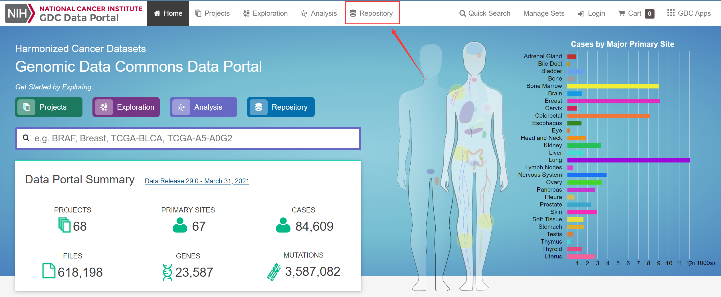
打开 GDC Portal(cancer.gov)，并进入 Repository（数据库）：
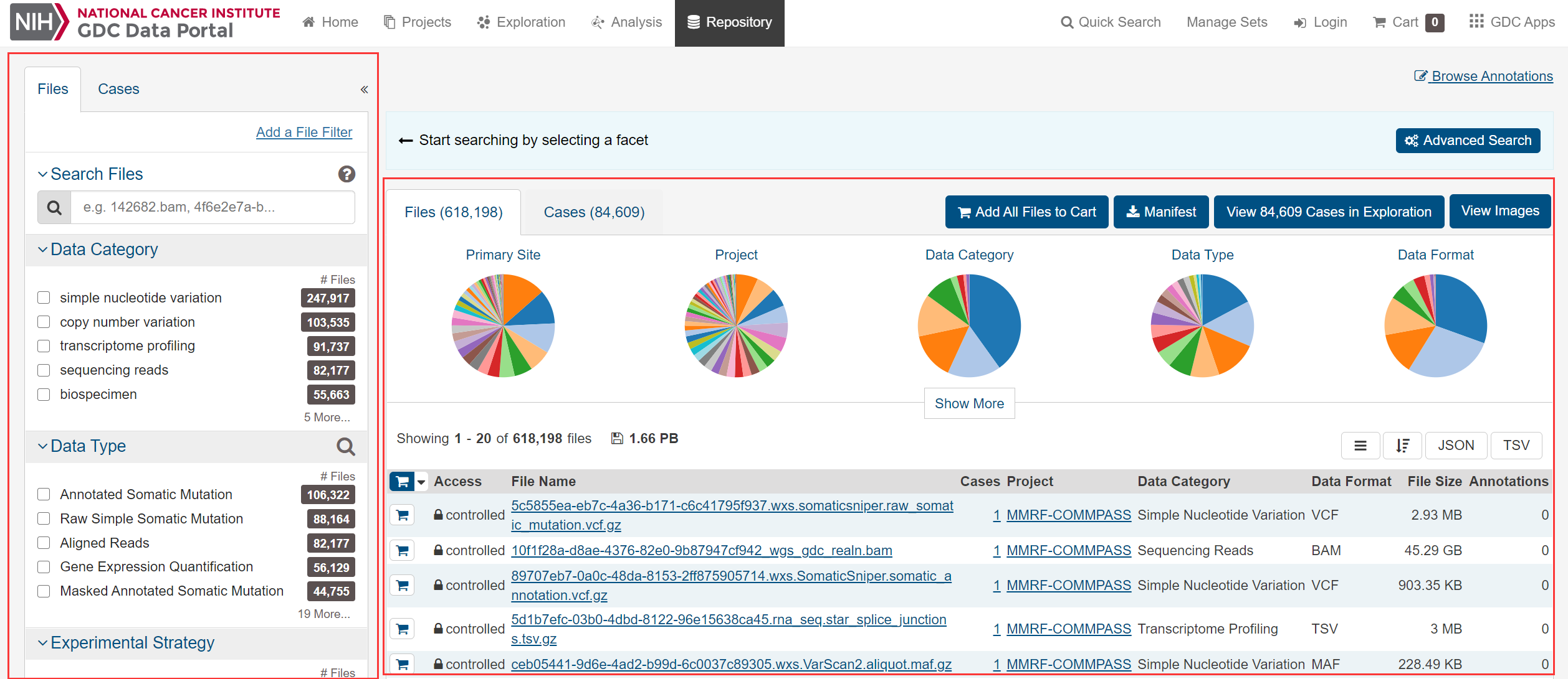
image-20210404220437260.png
如图，左侧是筛选和搜索区域，右侧是筛选后的结果：
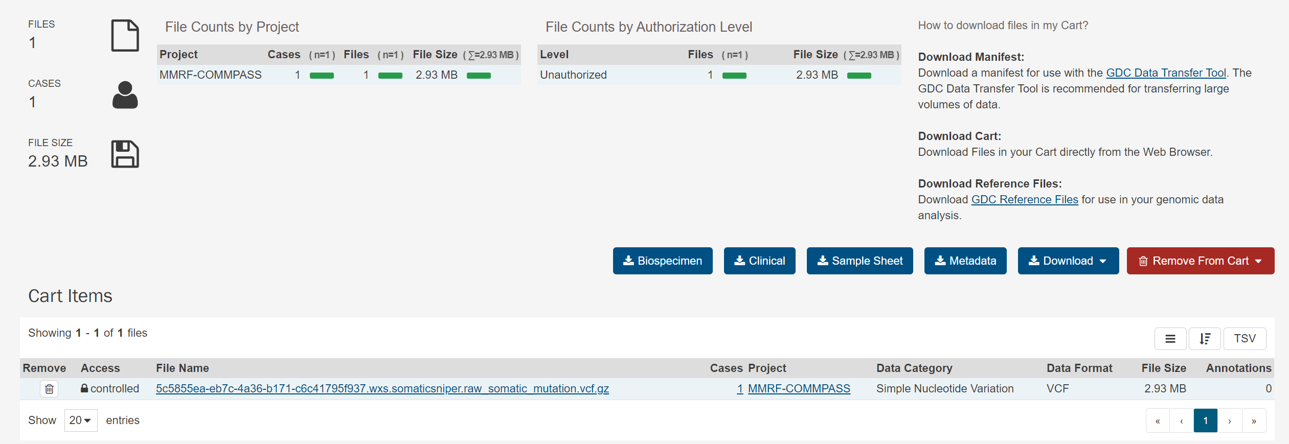
image-20210404220603208.png
筛选后可以将需要的结果加入购物车（Cart），然后进入购物车下载：
image-20210404220653949.png
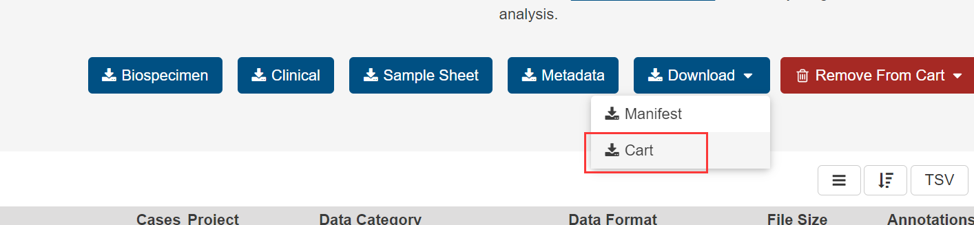
image-20210404220725436.png
如图所示，有 5 个下载选项，分别对应这个文件相关的信息（例如提供样品的病人的信息，下载的文件清单等等）：
image-20210404220737408.png

下面按照上面的通用步骤在 TCGA 数据库中获取两类数据：

TCGA-LGG 中的转录数据，作为原始数据，进行差异分析；
TCGA-LGG 中的临床数据，用于整理转录数据，通过临床数据我们将病人分为 TMZ 耐药和不耐药两组，以便进行差异分析；

获取转录数据

首先在上述第 2 步的基础上，设置筛选器。
先切换到 Case 选项卡，设置对病例的筛选：
1. Program 选择 TCGA（显然）；
2. Project 选择 TCGA-LGG（即 TCGA 中的 LGG 样本）；
3. 此时应该只有一种 Disease ，即 Gliomas（选不选无所谓）；
然后切换到 File 选项卡，挑选我们关心的数据：
1. Experimental Strategy 选择 RNA-Seq（即 RNA 测序数据）；
2. Workflow Type 选择 HTSeq - Counts（即原始的 counts 数据，因为我们后面使用的 DESeq2 工具自带有数据处理的功能，不需要我们预先对数据进行 FPKM 等操作）；
将筛选出的样本一键全部加入购物车，切换到 Cart 页面下载：
- 下载全部 Counts 数据：
  image-20210404233450091.png
- 然后下载元数据 Metadata：
  image-20210404234215243.png
  （下面整理文件会用到）
将刚刚下载的这两个文件放到一个文件夹中。

获取临床数据

和上面的步骤大同小异，Case 处的筛选条件相同，File 处设置为：
1. Data Category：clinical（筛选临床信息）；
2. Data Format：bcr biotable （Biotable 数据格式，即所有病人同时在一张表格里，方便整理）；
然后把筛选出来的 6 个文件加购物车下载即可，这次不需要 Metadata 了。

整理数据

下载后的数据不能直接使用，必须进行整理。

合成转录信息的总表

如图，这个 Counts 数据下载后在一个压缩包里面，而每个样本都是单独的一个文件夹，

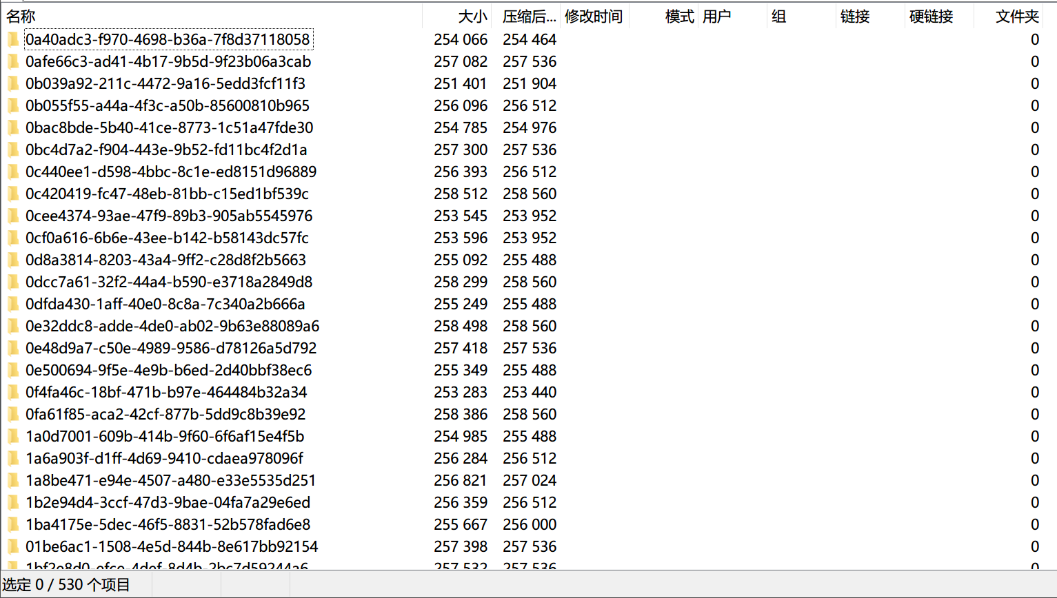
更糟糕的是，每个文件夹里面又是一个压缩包，没有直接能用的数据，更没有汇总好的表格。

所以这里使用 Python 脚本进行汇总：

# GenerateFiles.py: Unzip and move all the counts file into one folder.
# Note: Path below need replacing according to your own conditions!
# Made by Leo Lee (https://naiv.fun)

import os, re, gzip, time

os.chdir(r'C:\Users\leo\Desktop\大创\TCGA\data')
print("Current working path: " + os.getcwd())

dstPath = r'.\sample'
if os.path.exists(dstPath) == False:
    os.mkdir(dstPath)

cnt = 0
for root, dirs, files in os.walk("."):
    if root != dstPath:
        for i in files:
            if i.endswith(".gz") == True:
                print("Copying " + i)
                os.system("copy {} {}".format(root + '\\' + i, dstPath + '\\' + i))
                cnt += 1
print("Total copied: " + str(cnt) + " item(s).")

time.sleep(3)

cnt = 0
for root, dirs, files in os.walk(dstPath):
    for i in files:
        if i.endswith(".gz") == True:
            print("Unzipping and removing: " + root + "\\" + i)
            with gzip.open(root + "\\" + i, "rb") as f_in:
                with open(root + "\\" + i[:-3], "wb") as f_out:
                    f_out.write(f_in.read())
            os.remove(root + "\\" + i)
print("Total unzipped: " + str(cnt) + " item(s).")

这段代码完成后会在原地生成一个 sample 文件夹，里面是解压后的所有样本的 counts 数据，但是还没有被汇总。

接下来用 Python 脚本汇总，注意这里使用了 Pandas 库，需要预先安装好（安装过程略）。

# MergeData.py: match the samples with metadata and merge them into one table.
# Note: Path below need replacing according to your own conditions!
# Made by Leo Lee (https://naiv.fun)

import os, json, pandas as pd

json_name = "metadata.cart.2021-01-26.json"
root_path = r'C:\Users\leo\Desktop\大创\TCGA\data'
sample_path = r'C:\Users\leo\Desktop\大创\TCGA\data\sample'

os.chdir(root_path)
print("Current working path: " + os.getcwd())
metadata = 0
with open(json_name) as f:
    metadata = json.load(f)
print("Read " + str(len(metadata)) + " metadata.")

os.chdir(sample_path)
print("Current working path: " + os.getcwd())
print("Merging data...")

merged_df = pd.DataFrame()
for sample_dic in metadata:
    barcode = sample_dic["associated_entities"][0]["entity_submitter_id"]
    file_name = sample_dic["file_name"][:-3]
    sample_df = pd.read_table(sample_path + '\\' + file_name, names = [barcode], index_col = 0)
    merged_df = pd.concat([merged_df, sample_df], axis = 1)

print("Data has been merged, results are as follow: ")
print(merged_df)

merged_df.to_csv(root_path + '\\Results.csv')
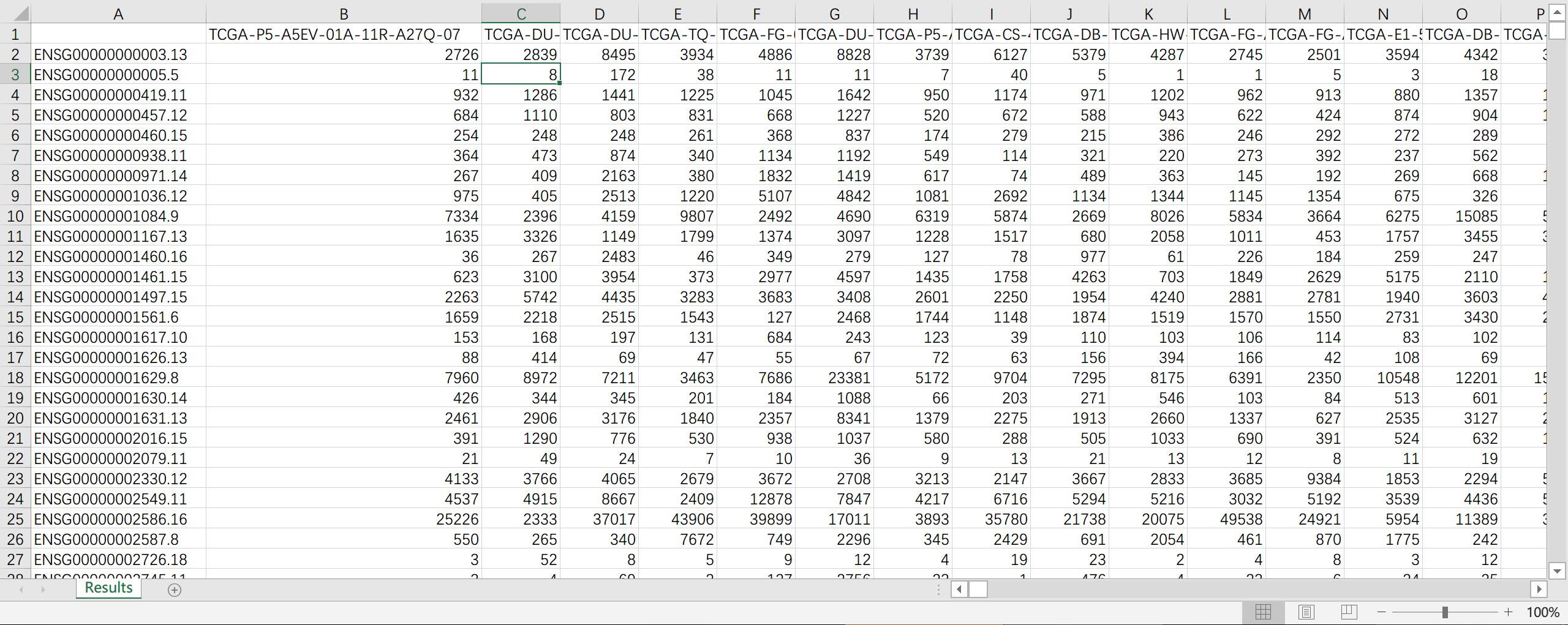
print("Results are saved to: " + root_path + '\\Results.csv')

运行之后会在原地生成 Results.csv，内容就是所有 Counts 数据的汇总，其中每列代表每个样本，每行代表不同基因：

通过临床信息分组

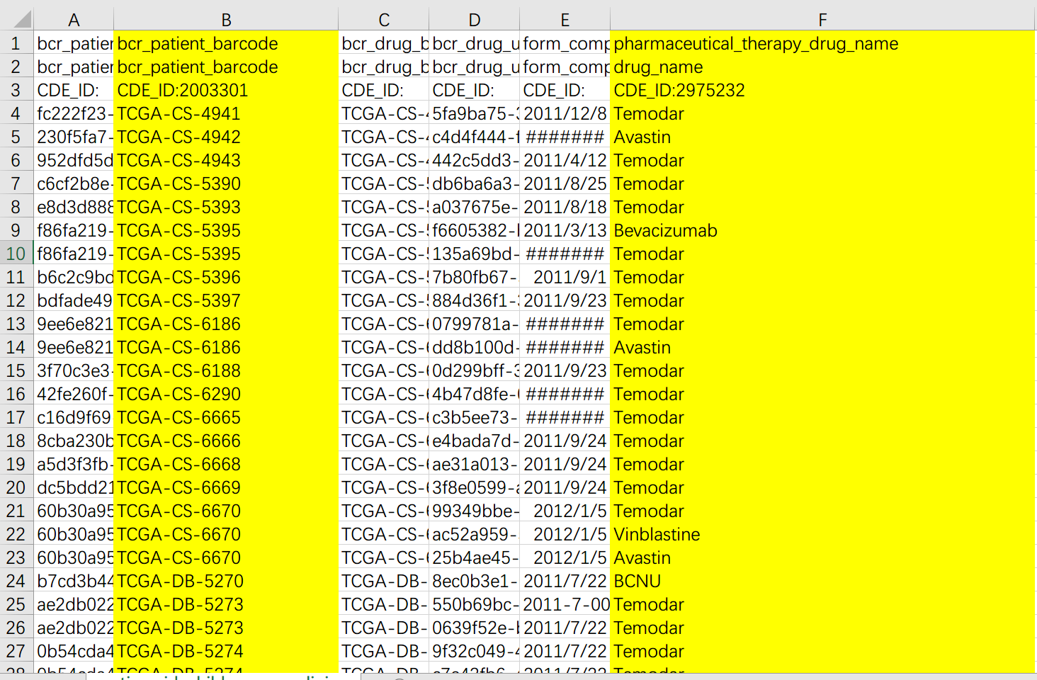
这里我们重点关注临床数据中后缀为 clinical_drug_lgg.txt 和 clinical_follow_up_v1.0_lgg.txt 的文件，前者是用药信息的表格，后者是随访信息的表格。

如下是 Drug 信息中我们重点关注的两列，前面的是病人 ID，后面的是药物治疗中使用的药物。

这里需要特别注意："Temozolomide", "temozolomide", "Temodar", "temodar"，都是 TMZ，我们要做的就是先把所有用过TMZ 的人筛选出来。

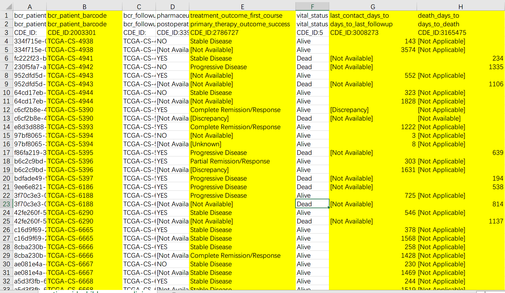
筛选出来之后，我们再来看 Follow-up 信息，其中比较有用的是以下四列（为了展示方便我删除了一部分没有用到的列）。

从左到右分别是（我的理解很粗浅，翻译不一定准确）

病人 ID；
第一疗程后的病人状况。这里的取值，除去无效数据之外共有四种，只有 Progressive Disease 可以被认为是耐药，我们就从这里入手，将病人分为耐药和不耐药两组（这个过程中数据无效的病人被剔除了）。
最后一次联系日期；
死亡日期；

需要注意的是，最后两列中通常只有一列有数据（貌似两个是互斥的），我们将两列中有数据的一个作为有效的日期，保存下来。

另外，我们会发现同一个病人可能有多次随访，每次随访他时疗效可能还不同，给我们分组带来迷惑和困难，例如：

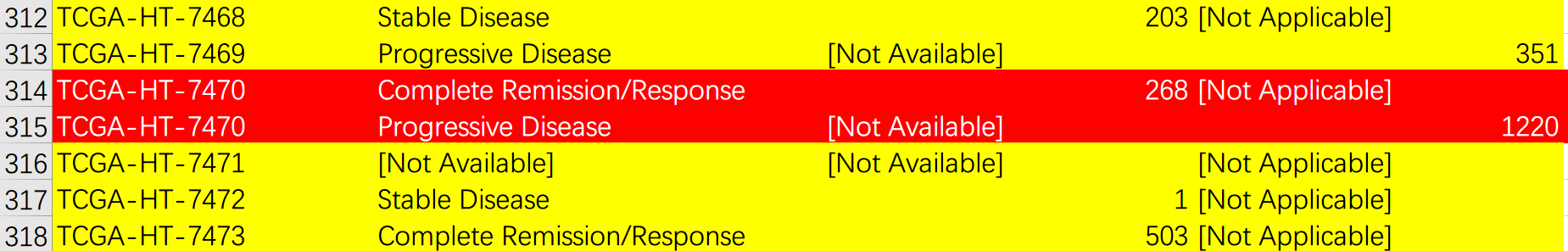
我们的解决方案是，按照日期对每个病人的随访记录进行排序，统一取靠前的第一条作为有效数据。

上面的操作很繁琐，我们继续通过 Python 脚本实现：

# selectDrug.py: Grouping patients by standard mentioned above.
# Note: Path below need replacing according to your own conditions!
# Made by Leo Lee (https://naiv.fun)

import os, pandas as pd

sample_path = r"C:\Users\leo\Desktop\大创\TCGA\Clinical\sample"
drug_filename = r"nationwidechildrens.org_clinical_drug_lgg.txt"
follow_filename = r"nationwidechildrens.org_clinical_follow_up_v1.0_lgg.txt"

# find drug users
drug_name = ["Temozolomide", "temozolomide", "Temodar", "temodar"]
drug_df = pd.read_table(sample_path + '\\' + drug_filename,
                        header=0, index_col=None, usecols=[1, 5])
drug_user = drug_df[drug_df.pharmaceutical_therapy_drug_name.isin(
    drug_name)]["bcr_patient_barcode"]

# clean illegal data
illegal_data = ["[Not Available]", "[Unknown]", "[Discrepancy]"]
follow_df = pd.read_table(sample_path + '\\' + follow_filename,
                          header=0, index_col=None, usecols=[1, 9, 11, 12])
follow_df = follow_df[follow_df.bcr_patient_barcode.isin(drug_user)]
follow_df = follow_df[~follow_df.treatment_outcome_first_course.isin(
    illegal_data)]

# merge date
follow_df["date"] = None
follow_df.reset_index(drop=True, inplace=True)
for i in range(0, len(follow_df)):
    if str(follow_df.iloc[i]["last_contact_days_to"]).startswith("["):
        try:
            follow_df.loc[i, "date"] = int(follow_df.iloc[i]["death_days_to"])
        except ValueError:
            follow_df.loc[i, "date"] = 0
    else:
        follow_df.loc[i, "date"] = int(
            follow_df.iloc[i]["last_contact_days_to"])
follow_df.drop(labels=["last_contact_days_to",
                       "death_days_to"], axis=1, inplace=True)

# generate two samples
follow_df.sort_values(by="date", axis=0, inplace=True, ignore_index=True)
sample1 = follow_df.drop_duplicates(
    subset="bcr_patient_barcode", ignore_index=True)
sample2 = follow_df.drop_duplicates(
    subset="bcr_patient_barcode", keep="last", ignore_index=True)

# group the users and print out

PD_user = sample1[sample1.treatment_outcome_first_course ==
                     "Progressive Disease"]
not_PD_user = sample1[(sample1.treatment_outcome_first_course !=
                         "Progressive Disease")]

PD_user.to_csv("TMZ_R_sample1.csv")
not_PD_user.to_csv("TMZ_NR_user_sample1.csv")

PD_user = sample2[(sample2.treatment_outcome_first_course ==
                     "Progressive Disease")]
not_PD_user = sample2[(sample2.treatment_outcome_first_course !=
                         "Progressive Disease")]

PD_user.to_csv("TMZ_R_sample2.csv")
not_PD_user.to_csv("TMZ_NR_user_sample2.csv")

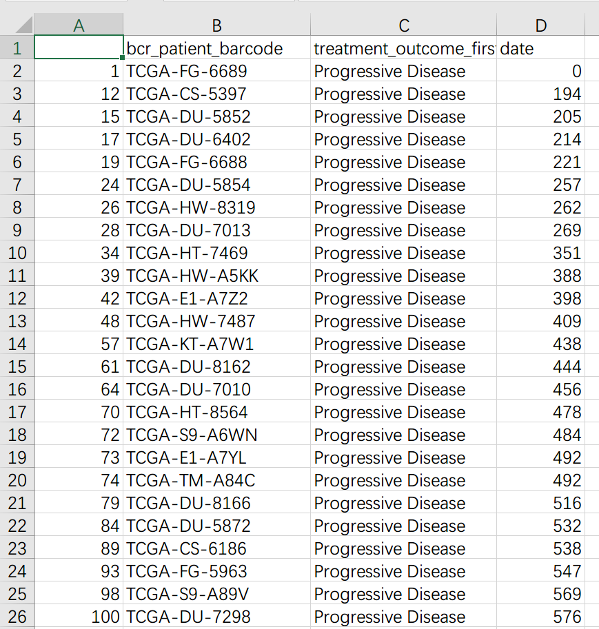
脚本运行后在原地生成 TMZ_R_sample1.csv, TMZ_NR_sample1.csv。其中 R 为耐药、NR 为不耐药，另外后缀 sample1 代表按照日期靠前的记录分组后的结果，为了严谨起见，本脚本还会按照靠后的记录分组一次，结果保存在后缀为 sample2 的表格中。效果如下：

不耐药组（NR）：

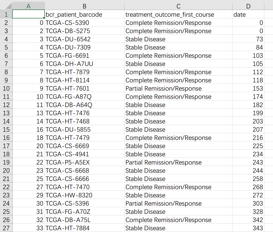
耐药组（R）：

整合转录信息和临床信息

以上操作仅仅完成了病人的分组，下面要按照病人的分组把转录数据也分成两个文件。

将整理数据所得的文件 Results.csv, TMZ_NR_sample1.csv, TMZ_R_sample1.csv 置于同级目录下，下面继续使用 Python 脚本处理：

# generate.py: Divide the counts data into two group according to previous results.
# Note: Path below need replacing according to your own conditions!
# Made by Leo Lee (https://naiv.fun)

import pandas as pd

PD_user = pd.read_csv("TMZ_R_sample1.csv", usecols=[1])
not_PD_user = pd.read_csv("TMZ_NR_sample1.csv", usecols=[1])
raw = pd.read_csv("Results.csv", index_col=0)

PD_counts = pd.DataFrame()
not_PD_counts = pd.DataFrame()

for name in raw:
    if int(name[13:15]) > 10:
        continue
    if name[:12] in list(PD_user["bcr_patient_barcode"]):
        PD_counts[name] = raw[name]
    elif name[:12] in list(not_PD_user["bcr_patient_barcode"]):
        not_PD_counts[name] = raw[name]

PD_counts.to_csv("R_counts.csv")
not_PD_counts.to_csv("NR_counts.csv")

运行完毕后生成两个文件，R_counts.csv 与 NR_counts.csv，前者是耐药组的 Counts 数据，后者是不耐药组的 Counts 数据。

差异分析

完成以上工作后，终于进入差异分析环节。

正确设置目录

回顾以上工作，我们新建一个文件夹，里面只放入 R_counts.csv 与 NR_counts.csv，以便下一步编写 R 语言脚本。

安装 DESeq2

生物信息学软件仓库：Bioconductor - Home

安装方法：Bioconductor - DESeq2

运行 R 脚本

将脚本放入刚刚新建的文件夹，然后运行：

# diff.r: Differ the genes between two groups.
# Note: Path below need replacing according to your own conditions!
# Made by Leo Lee (https://naiv.fun)

setwd("C:\\Users\\leo\\Desktop\\大创\\TCGA\\differ\\sample1")

pd_counts =  read.csv("R_counts.csv", row.names = 1, header = TRUE)
not_pd_counts = read.csv("NR_counts.csv", row.names = 1, header = TRUE)

counts = cbind(pd_counts, not_pd_counts)

DesGroup = c(rep("control", 152), rep("case", 76))

colData = data.frame(row.names = names(counts),
                     condition = factor(DesGroup,
                                        levels = c("control", "case")))
library(DESeq2)

dds = DESeqDataSetFromMatrix(countData = counts, colData = colData, design = ~ condition)

dds = DESeq(dds)

sizeFactors(dds)

res = results(dds)

res = as.data.frame(res)

res = cbind(rownames(res), res)

colnames(res) = c("gene_id", "baseMean", "log2FoldChange", "lfcSE", "stat", "pval", "padj")

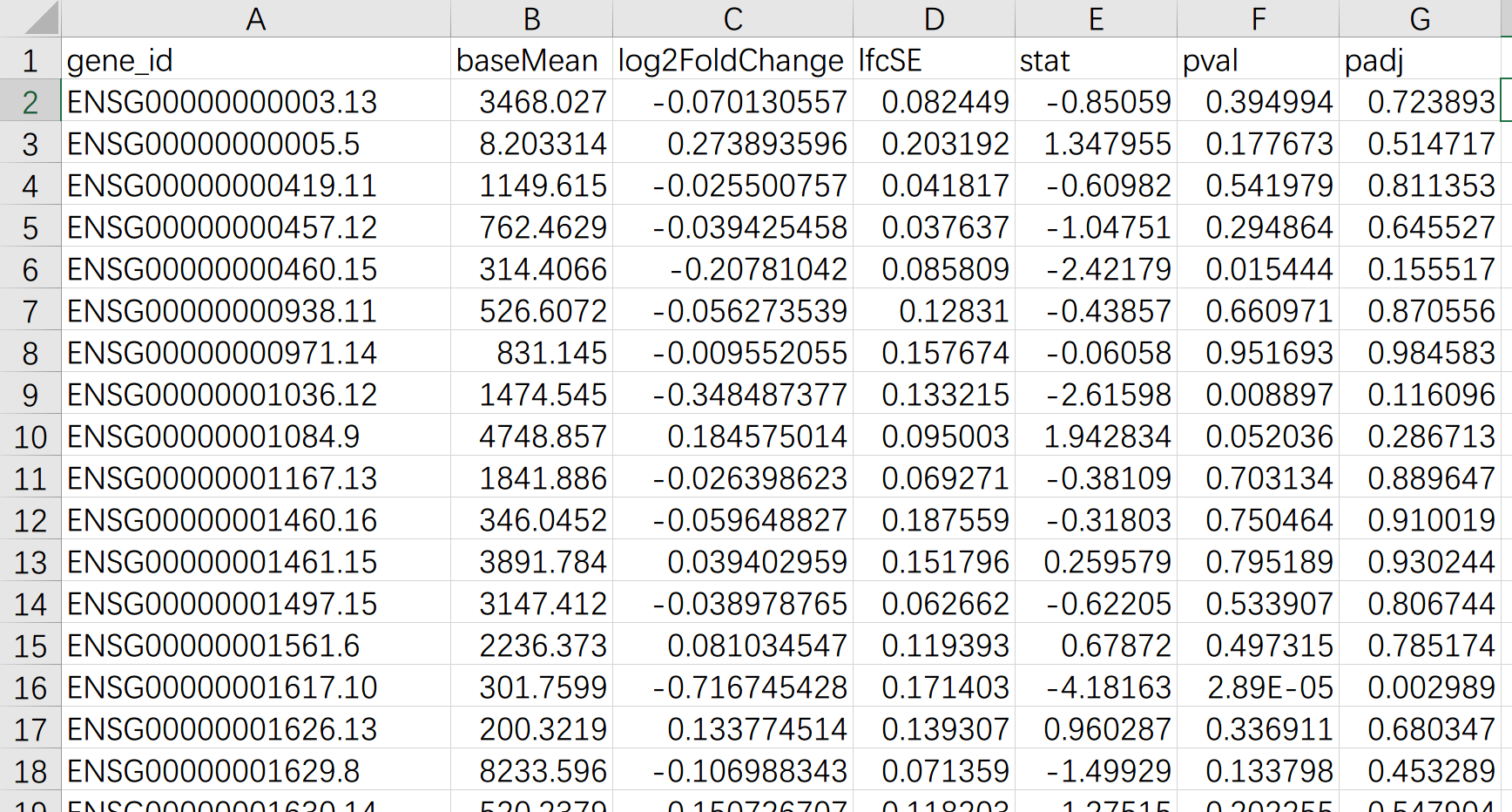
write.table(res, "DESeq2.gene.diff.csv", sep = ",", col.names = TRUE, row.names = FALSE, quote = FALSE, na = "")

运行完毕后，会在原地生成 DESeq2.gene.diff.csv，内容如下，每行是基因 ID，每列代表一个统计学数据（我也不懂），接下来我们通过这些数据筛选出差异较显著的基因。

筛选显著的差异基因

这里我们利用 Python 脚本以 $padj < 0.05$ 且 $|log2FoldChange| > 0.58$ 为标准，筛选差异显著的基因：

# filter.py: Filter genes according to standard mentioned above.
# Note: Path below need replacing according to your own conditions!
# Made by Leo Lee (https://naiv.fun)

import pandas as pd

genes = pd.read_csv("DESeq2.gene.diff.sample1.210214.csv", header = 0, index_col=None)

gene_list = []

for i in range(len(genes)):
    if genes.padj[i] < 0.05 and abs(genes.log2FoldChange[i]) > 0.58:
        gene_list.append(str(genes.gene_id[i]).split(sep='.')[0])
 
gene_list = pd.DataFrame(data = {"gene_id" : gene_list})
gene_list.to_csv("Diff_genes_1.5.csv")

脚本执行完毕后，在原地生成 Diff_genes_1.5.csv，如图所示：

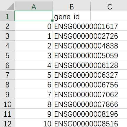
即为我们筛选得出的差异基因名单。

基因富集

基因功能富集分析，即借助各类数据库和分析工具进行统计分析，挖掘在数据库中与我们要研究的生物学问题具有显著相关性的基因功能类别。

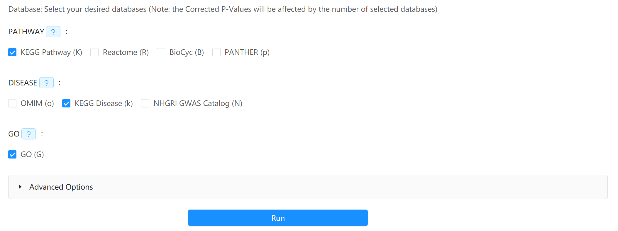
这里我们借助 KOBAS 工具对 KEGG 数据库进行通路富集分析。

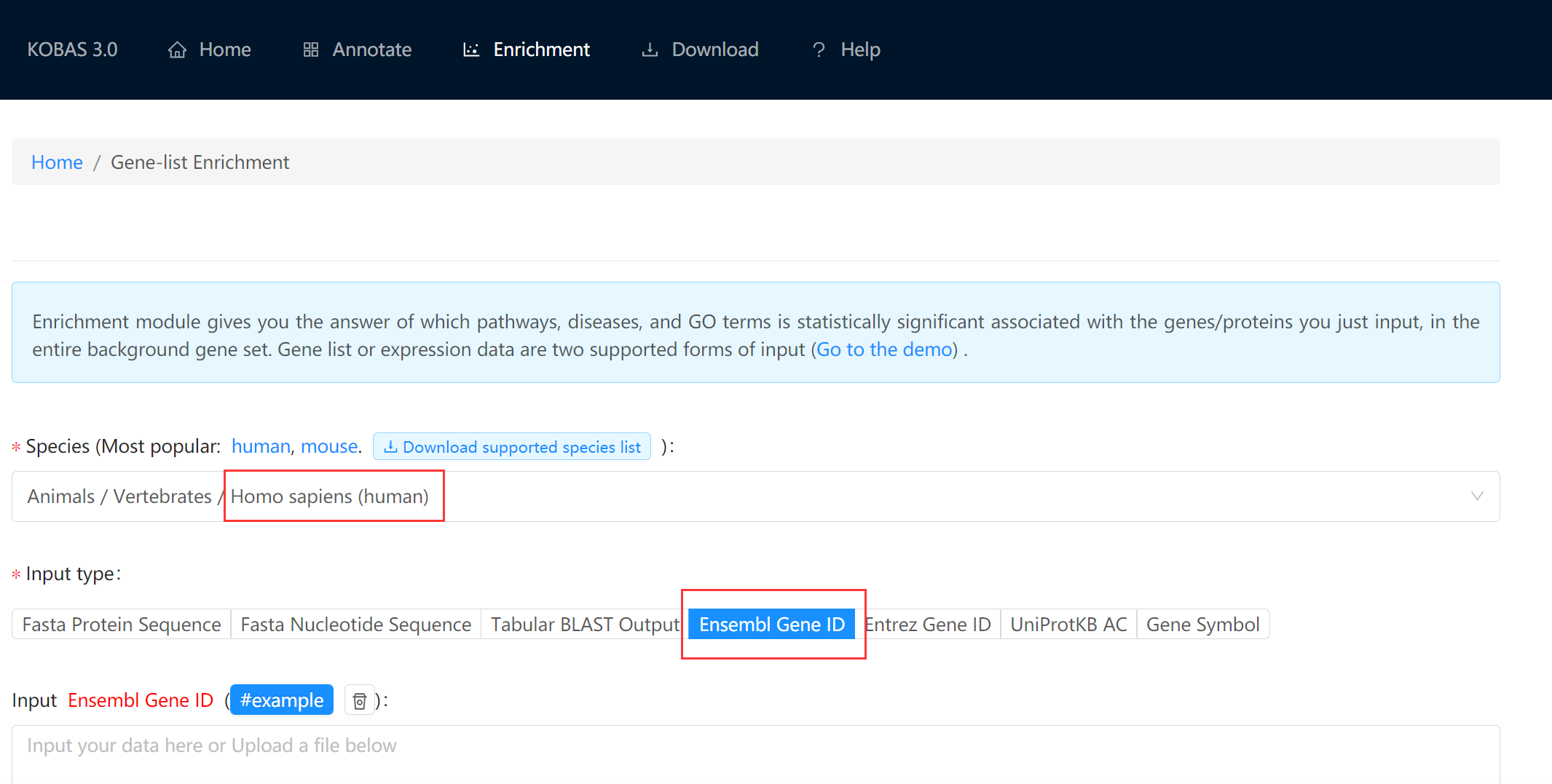
直接将上一步中得到的差异基因列表粘贴到网站上，选择人类，然后进一步选择 KEGG Pathway 分析:

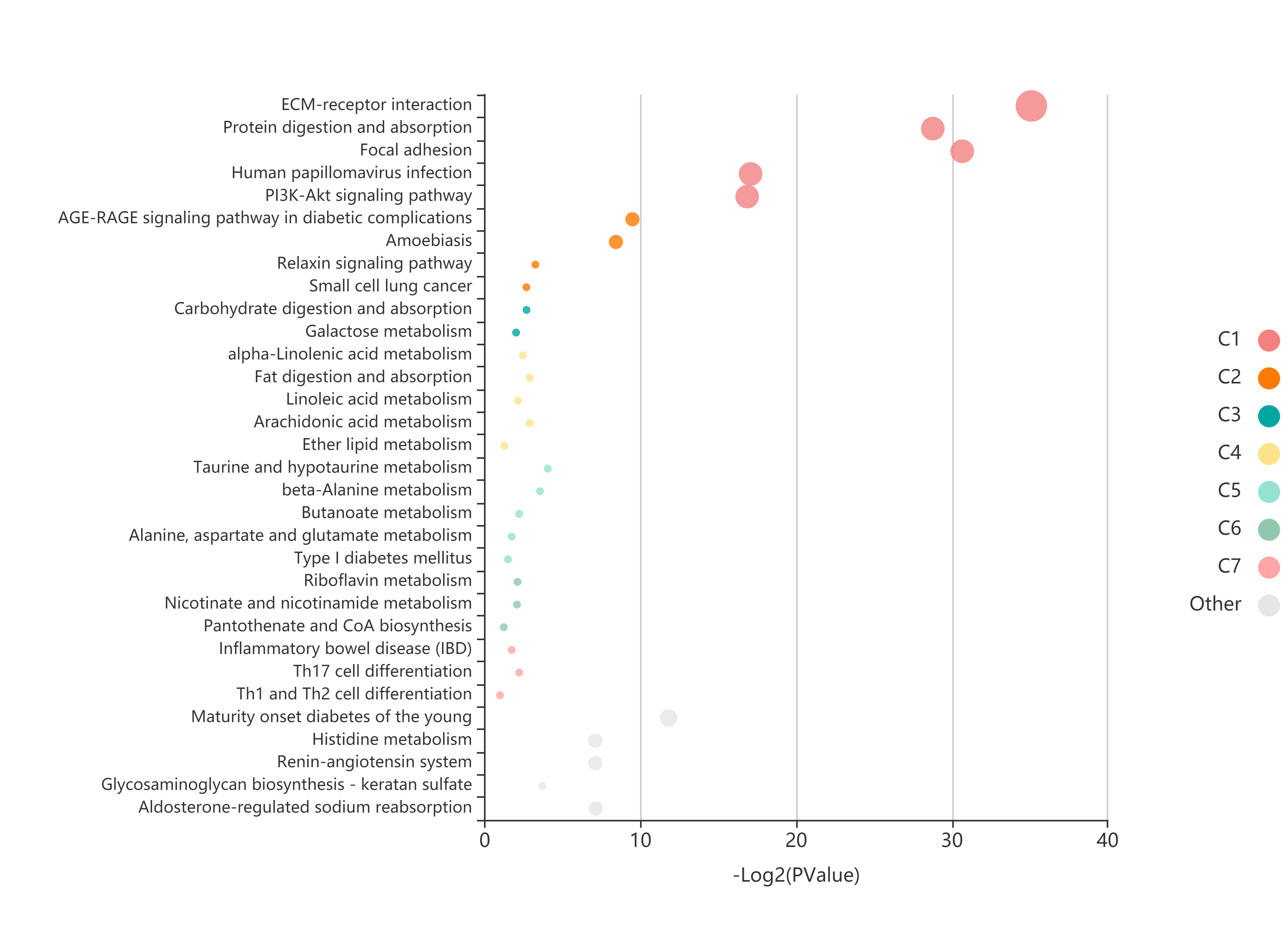
等候一段时间后，即可获取结果，包括比对后的表格结果，以及生成的气泡图，例如：

后记

本篇文章重点仅在于介绍工具的使用，学术方面的问题恐怕我难以解释。由于笔者并非来自生物信息学专业，仅有半个月左右自行摸索的经历，文中难免有错讹之处，还望读者不吝指正。最后还要特别感谢导师的指导和帮助，让我这个“行外人”完成本次基因差异分析工作。

参考资料

行外人的一次 TCGA 数据库基因差异分析

获取数据

获取转录数据

获取临床数据

整理数据

合成转录信息的总表

通过临床信息分组

整合转录信息和临床信息

差异分析

正确设置目录

安装 DESeq2

运行 R 脚本

筛选显著的差异基因

基因富集

后记

参考资料

添加新评论

已有 2 条评论

行外人的一次 TCGA 数据库基因差异分析

获取数据

获取转录数据

获取临床数据

整理数据

合成转录信息的总表

通过临床信息分组

整合转录信息和临床信息

差异分析

正确设置目录

安装 DESeq2

运行 R 脚本

筛选显著的差异基因

基因富集

后记

参考资料

记一次 Typecho 博客迁移的经历

解决 Typecho 无法上传图片的问题

添加新评论

已有 2 条评论